How to Improve the Accuracy of Inclination Measurement Using an Accelerometer

Typical Application of Tilt Measurement

This article discusses how to improve tilt measurement accuracy using an accelerometer like a combo part. Electric park brakes (EPBs) are used on passenger vehicles to hold the vehicle stationary on graded and flat roads. This is accomplished by measuring the inclination using a single-axis or dual-axis accelerometer. Typically, an x-, y-, or z-axis low-g accelerometer is placed in a dedicated module of an EPB control unit. Now, more and more vehicles have an electronic stability control (ESC)function with a combined low-g accelerometer and gyroscope in a single chip. This is done to prevent the vehicle from side slipping and rolling over, and now ESC function is demanded world-wide through legislation. If tilt measurement is accomplished by a combo part (single-chip, combined accelerometer and gyroscope), then it is not necessary to have a standalone EPB module on the vehicle, which would significantly reduce the cost of the car. Because a combo part is typically used for ESC, it’s not optimised for tilt sensing, and sometimes, the accuracy of the tilt measurement by a combo part could not meet the accuracy requirement. Because a combo is xy-axis or xyz-axis, it typically uses the x-axis for tilt measurement and some of the traditional low-g accelerometers in EPB modules use the z-axis, because it’s installed vertically in the engine compartment. The sensing axis should be placed perpendicular to gravity to achieve better accuracy - this will be discussed later.

For tilt measurement on a vehicle, it’s very important to evaluate the accuracy. Imagine that your car is parking on absolutely flat ground, so the angle calculated by the accelerometer should be 0°. If your car is parking on a ramp, the inclination should be accurately detected so that the braking system would be actuated correctly.

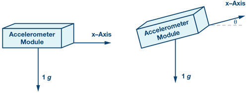
So

Where:

AOUT is the output of the accelerometer in g.

θ is the inclination of the ramp in degrees.

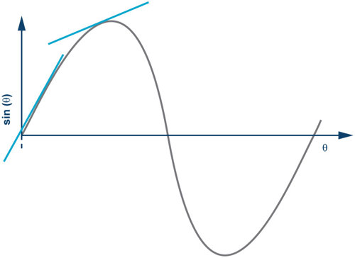
Because sin θ is a nonlinear function, the relationship between AOUT and θ is nonlinear and it has the best linearity near zero, which means it has the best measuring accuracy. As θ increases, the measuring accuracy degrades. That’s why the sensing axis should be placed perpendicular to gravity, because the road slope grade will be close to zero.

For tilt measurement on a vehicle, it’s not necessary to consider the system with full ramp slope. The vast majority of ramp slope on the road in the real world would not exceed 30°. We only have to analyse the accuracy of contributions within the range of ±30°.

There are several contributions that would affect system-level measurement accuracy:

• Sensitivity error and initial absolute offset
• Nonlinearity
• Total offset variation from initial absolute offset
• Noise

Sensitivity Error and Initial Absolute Offset

Sensitivity Error

Sensitivity is the slope of the transfer function measured of inputs-outputs, usually at +1g and –1g. Sensitivity error is the part to part deviation of sensitivity. For example, some accelerometers’ maximum sensitivity is 3%.

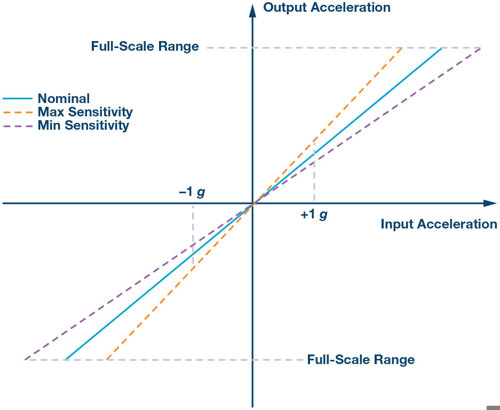
Initial Absolute Offset

The offset within the range is around 25°C; for example, 25°C ± 5°C, measured immediately after completion of the module’s manufacture. The initial absolute offset denotes the standard deviation of the measured offset values across a large population of devices.

Two-Point Calibration

For tilt measuring applications, the two main errors come from offset error and sensitivity error. These two errors lead to an unacceptable sensing result, so they should not be neglected. If we want to remove these two parts of error, the output of acceleration should be calibrated. Typically, there is a one-time calibration for offset and sensitivity of tilt measurement. If the offset and sensitivity error is considered, the relationship of input vs. output of the accelerometer is:

Where:

AOUTPUT is the offset error in g.

Gain is the gain of the accelerometer, the ideal value is 1.

AACTUAL is the real acceleration applied on the accelerometer in g.

There are two basic calibration techniques; one is single-point calibration. This calibration is done by applying a 0g field on the accelerometer and then measuring the output. This kind of calibration could just be used for calibrating offset error and gain error could not be calibrated. Then, the resulting output in a 0g field is subtracted from the real output value to remove the offset error.This is an easy method for calibration, but not for accuracy, because there’s still sensitivity error. Another way is 1g flip calibration, which would use two-point calibration at +1g and –1g, and in each field of +1g and –1g measure the acceleration output as below:

where the offset, AOFFSET, is in g.

From this two-point information, offset and gain could be resolved as follows:

Where the +1g and −1g measurements, A+1 g and A–1 g, are in g.

After this one-time calibration, the actual acceleration could be calculated by following this equation, each time removing theoffset and sensitivity error.

Nonlinearity

The nonlinearity of the device is the maximum deviation of the measured acceleration (AMEA) and the ideal linear output acceleration (AFIT). The data-set of the acceleration measurement should include the full-scale range of the accelerometer. It’s measured as Max(|AMEA – AFIT|).

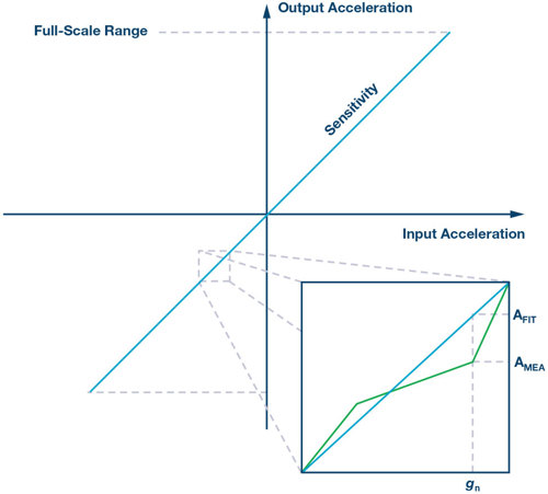
Where:

AMEA is measured acceleration at a defined gn.

AFIT is predicted acceleration at a defined gn.

Most accelerometer or combo parts have nonlinearity over a given input accelerometer range - for example, a range of 30mg ± 2g. For tilt measurement applications, the input ramp slope is within ±30°, which means the output acceleration range is within ±500mg (±1g × sin 30°), so the nonlinearity within this range should be reassessed. Because the nonlinearity is not linear across the whole input range, it’s difficult to evaluate this part of error accurately and quantitatively. However, because the data sheet for this part is usually very conservative for a nonlinearity of 30mg with an input range of ±2g, it would be more reasonable to use 10mg for the error calculation within ±500mg.

Total Offset Variation from Initial Absolute Offset

Total offset variation from initial absolute offset is the maximum deviation of the offset as induced by temperature, stress, and aging effects. This deviation is measured relative to the initial absolute offset for a given device. This is the main contribution to the total error of accuracy.

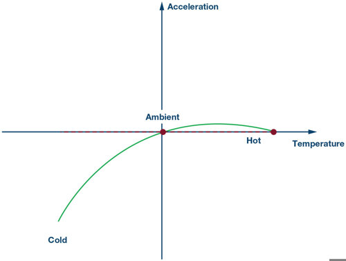
Among all these factors like temperature, stress, aging, etc., variation vs. temperature accounts for the major percentage of total offset variation. Typically, the variation vs. temperature curve is a second-order curve, which is typically a rotated parabola. Inorder to eliminate this part of error, a three-point calibration at the system level could be performed. For a given device, the output variation drift vs. temperature could be calibrated with the following steps.

Step 1:

The output response of the device is shifted by some value ΔN0. The first step in the temperature calibration process is to cancel out the offset at ambient.

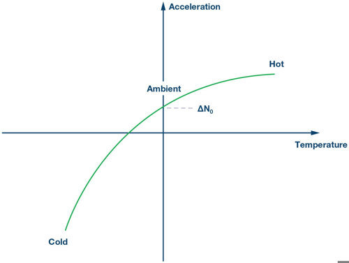
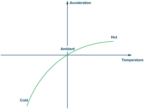
Step 2:

Next, the device is tested at a hot temperature and this new information is used to generate a linear equation for offset correction.

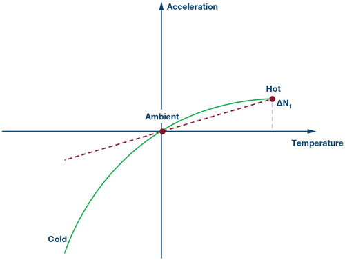
Step 3:

A second-order component is added to the existing equation in order to correct for the remainder of the offset. Assuming the second-order curve follows the equation below:

This is a second-order parabola formula and the rotation component has been cancelled through steps 1 and 2.

This second-order parabola has three solutions to this equation:

Then we could get tempco a, b, c.

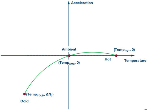
All the tempco information of ΔN0, ΔN1, ΔN2, a, b, c should be stored in the system’s non-volatile memory and an on-board temperature sensor is needed. The system would calibrate the accelerometer routinely after each power-on to ensure the cancellation of the variant drift vs. temperature.

Noise

A tilt measurement based on a single sample of data may not be reliable. Even if the accelerometer had zero noise, tilt measurements are being made while the car is on, so any or all vibration caused by the engine, passing vehicles, or the passengers shifting around within the car will all need to be mitigated. The best way to do this is to average the data for as long aspossible without falling below the minimum data rate requirements. This averaging will reduce the rms noise.

Assuming we sample the noise, we get a per-sample variance of

Averaging a random variable leads to the following variance,

Since noise variance is constant at σ2,

Because random noise is subject to Gaussian distribution, rms noise is equivalent to the standard deviation of Gaussiandistribution. The minimum population within 6σ is 97%.

For example, if you are averaging every 100ms of data at 1kSPS, then a max rms noise = 0.4mg, meaning the calculation for peak noise at that point is only 2.4mg if we use 6σ as the distance from the mean.

The factors that you are multiplying the rms value by depend on the statistical needs of the mission profile for the part. For example, choosing 6 as the factor (peak-to-peak noise is 6 × rms noise) will impact the probability of a worst-case scenario happening during the part’s lifetime. RMS noise is a fixed value indicated in a product’s data sheet. It’s the standard deviation, which means it’s in the 1 sigma distribution. It cannot be used for the calculation as the containment limit within a 1 sigma distribution is only 68.26%. This is why we have to choose a higher factor to multiply the rms noise by. A larger factor will lead to better containment.

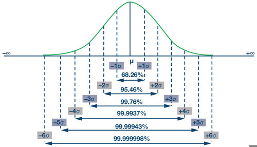
Theoretically, the factor that is multiplying the rms noise will determine the failure time during the algorithm’s lifetime because noise is a random variable over time. But while noise is not predictable, it can be calculated statistically.

Let’s say that an EPB module’s algorithm has an expected run-time of 146,000 (that is, 20 times per day for 20 years). If no failures are allowed over its lifetime, the maximum failure rate is 1/146,000 = 0.00068%.

According to the sigma level of Gaussian distribution (Figure 11), the sigma level of 6 generates 0.00034% defective percentage. Thus, choosing 6 as the rms multiplication factor corresponds to 146,000 × 0.00034% = 0.5 < 1. This means that statistically there won’t be any failure for the EPB module over a lifetime of 20 years.

We can summarise this as:

E is the expected times exceeding the worst case over lifetime, M is the lifetime running times, and r is the probability ofexceeding the worst case. Based on this, we can evaluate a reasonable factor by multiplying the rms noise.

Summary

Taking ADI’s ADXC1500/ADXC1501 (combined gyroscope and 2-axis/3-axis accelerometer) as an example, all the error contribution items are listed in Table 1 with or without calibration measures. We can assume total offset variation is the 2nd curve and variation over temperature accounts for 80% of its total offset variation. Also, take 6 as the factor multiplied by the maximum rms noise.

This combination of a gyroscope and tri-axis accelerometer enables many new applications, especially in automotive safety systems and industrial automation applications. Minimising these large error sources is mission critical to designing more reliable and accurate automotive safety systems, such as robust electronic stability control (ESC) and rollover detection. These build on traditional chassis control systems already in the vehicle, including the anti-lock braking system, traction control, and yaw control.

Table 1. Error Contributions With/Without Calibration

Analog Devices: www.analog.com

Acknowledgements

I’d like to thank my two colleagues, Matthew Hazel and Brian Larivee, for providing many useful thoughts in this article.

About the Author

Allen Fan [allen.fan@analog.com] is a field applications engineer with the ADI China Automotive Sales Team. He’s responsible for the support and promotion of radar, IMU, powertrain, and infotainment products in China. He received a bachelor’s degree in mathematics from Shan Dong University.